26. Stokes' Theorem
Let \(S\) be a nice surface in \(\mathbb{R}^3\) with a nice properly oriented boundary, \(\partial S\), and let \(\vec{F}\) be a nice vector field on \(S\). Then \[ \iint_S \vec{\nabla}\times\vec{F}\cdot d\vec{S} =\oint_{\partial S} \vec{F}\cdot d\vec{s} \] Each piece of the boundary of the surface must be traversed counterclockwise as seen from the tip of the normal vector to the surface.
d. Applications
1. Converting Line Integrals to Surface Integrals
Problems involving Stokes' Theorem have the potential to be confusing. When a problem asks you to compute the line integral \(\displaystyle \oint \vec{F}\cdot d\vec{s}\) using Stokes' Theorem, you really need to compute the surface integral \(\displaystyle \iint \vec{\nabla}\times\vec{F}\cdot d\vec{S}\). Conversely, when a problem asks you to compute the surface integral \(\displaystyle \iint \vec{\nabla}\times\vec{F}\cdot d\vec{S}\) using Stokes' Theorem, you really need to compute the line integral \(\displaystyle \oint \vec{F}\cdot d\vec{s}\). The good news is that Stokes' Theorem usually turns complicated integrals into relatively simple ones. Almost always you will be given the integral in its complex form, and it can be simplified by using Stokes' Theorem.
Stokes' Theorem is used to convert a line integral into a surface integral when taking the curl gives a simpler vector and/or the surface is easier than the boundary. These problems are discussed here. (Applications which go in the other direction are discussed on the next page.)
Compute \(\displaystyle \oint_{\partial S} \vec{F}\cdot d\vec{s}\) for \(\vec{F}=\langle y^3,z^2,x^4\rangle\) counterclockwise around the rectangle \(x=4\quad 0 \le y \le 3\quad 0 \le z \le 2\) as seen from the positve \(x\)-axis.
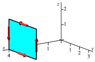
The integral is given to us as a line integral. We can simplify it by converting it into a region integral using Stokes' theorem since \(\vec{\nabla}\times\vec{F}\) is easier than \(\vec{F}\) and it is easier to integrate over a rectangle than four line segments.
We first parametrize the rectangle as: \[ \vec{R}(y,z)=(4,y,z) \quad \text{for}\quad 0 \le y \le 3 \quad 0 \le z \le 2 \] We compute the tangent and normal vectors: \[ \begin{array}{c} \\ \vec{e}_y= \\ \vec{e}_z= \end{array} \begin{vmatrix} \hat{\imath} & \hat{\jmath} & \hat{k} \\ (0 & 1 & 0) \\ (0 & 0 & 1) \end{vmatrix} \] \[ \vec{N}=\vec{e}_y\times\vec{e}_z =\hat{\imath}(1)-\hat{\jmath}(0)+\hat{k}(0) =\langle1,0,0\rangle \] Next we compute the curl of \(\vec{F}\), evaluate it on the surface and dot it into the normal: \[ \vec{\nabla}\times\vec{F}= \begin{vmatrix} \hat{\imath} & \hat{\jmath} & \hat{k} \\ \partial_x & \partial_y & \partial_z \\[2pt] y^3 & z^2 & x^4 \end{vmatrix} =\langle-2z,-4x^3,-3y^2\rangle \] \[ \left.\vec{\nabla}\times\vec{F}\right|_{\vec{R}(y,z)} =\langle-2z,-256,-3y^2\rangle \] \[ \left.\vec{\nabla}\times\vec{F}\right|_{\vec{R}(y,z)}\cdot\vec{N} =-2z \] Thus, the integral is \[\begin{aligned} \oint_{\partial S} \vec{F}\cdot d\vec{s} &=\iint_S \vec{\nabla}\times\vec{F}\cdot d\vec{S} =\int_0^2\int_0^3 \vec{\nabla}\times\vec{F}\cdot\vec{N}\,dy\,dz \\ &=\int_0^2\int_0^3 -2z\,dy\,dz =\left[\rule{0pt}{10pt}y\right]_0^3\left[\rule{0pt}{10pt}-z^2\right]_0^2=-12 \end{aligned}\] This was obviously easier than computing four line integrals.
Use Stokes' Theorem to compute the line integral \(\displaystyle \oint_{\vec r(\theta)} \vec F\cdot\,d\vec s\) for the vector vector field \(\vec F=\langle -xz,yz,z^2\rangle\) along the curve \(\vec r(\theta)=(2\cos\theta,2\sin\theta,4\sin\theta\cos\theta)\) as shown in the plot, traversed counterclockwise as seen from above.
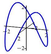
The curve lies on the surface \(z=xy\) which may be parametrized starting from cylindrical coordinates.
\(\displaystyle \oint_{\vec r(\theta)} \vec F\cdot\,d\vec s =\iint_S \vec{\nabla}\times\vec{F}\cdot d\vec{S}=8\pi\)
We want to use Stokes' Theorem to convert the line integral into a surface integral. So we need to have a surface for which the given curve is the boundary. Notice the curve lies on the surface \(z=xy\) which may be parametrized starting from cylindrical coordinates: \[ \vec R(r,\theta)=(r\cos\theta,r\sin\theta,r^2\sin\theta\cos\theta) \] And the given curve is obtained by setting \(r=2\). So the bounds on the parameters are \(0 \le r \le 2\) and \(0 \le \theta \le 2\pi\).
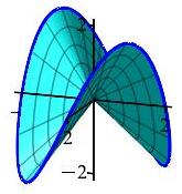
So the integral is: \[ \oint_{\vec r(\theta)} \vec F\cdot\,d\vec s =\iint_S \vec{\nabla}\times\vec{F}\cdot d\vec{S} =\int_0^{2\pi}\int_0^2 \left.\vec{\nabla}\times\vec{F}\right|_{\vec{R}(r,\theta)} \cdot\vec{N}\,dr\,d\theta \] The normal to the surface is: \[\begin{aligned} \vec{N}&=\vec{e}_r\times\vec{e}_\theta =\begin{vmatrix} \hat{\imath} & \hat{\jmath} & \hat{k} \\ (\cos\theta & \sin\theta & 2r\sin\theta\cos\theta) \\ (-r\sin\theta & r\cos\theta & r^2(\cos^2\theta-\sin^2\theta)) \end{vmatrix} \\ &=\hat{\imath}\,[\,r^2(\cos^2\theta\sin\theta-\sin^3\theta)-2r^2\sin\theta\cos^2\theta\,] \\ &\quad-\hat{\jmath}\,[\,r^2(\cos^3\theta-\sin^2\theta\cos\theta)+2r^2\sin^2\theta\cos\theta\,] \\ &\qquad+\hat{k}\,[\,r\cos^2\theta+r\sin^2\theta\,] \\ &=\hat{\imath}\,[\,-r^2(\cos^2\theta\sin\theta+\sin^3\theta)\,] \\ &\quad-\hat{\jmath}\,[\,r^2(\cos^3\theta+\sin^2\theta\cos\theta)\,] +\hat{k}\,[\,r\,] \\ &=\langle-r^2\sin\theta,-r^2\cos\theta,r\rangle \end{aligned}\] We compute the curl of \(\vec{F}=\langle -xz,yz,z^2\rangle\), evaluate it on the surface and dot it into the normal: \[ \vec{\nabla}\times\vec{F}= \begin{vmatrix} \hat{\imath} & \hat{\jmath} & \hat{k} \\ \partial_x & \partial_y & \partial_z \\ -xz & yz & z^2) \end{vmatrix} =\langle -y, -x, 0 \rangle \] \[ \left.\vec{\nabla}\times\vec{F}\right|_{\vec{R}(r,\theta)} =\langle -r\sin\theta, -r\cos\theta, 0 \rangle \] \[\begin{aligned} \left.\vec{\nabla}\times\vec{F}\right|_{\vec{R}(r,\theta)}\cdot\vec{N} =r^3\sin^2\theta+r^3\cos^2\theta =r^3 \end{aligned}\] So the integral is: \[\begin{aligned} \oint_{\vec r(\theta)} \vec F\cdot\,d\vec s &=\int_0^{2\pi}\int_0^2 r^3\,dr\,d\theta &=2\pi\left[\dfrac{r^4}{4}\right]_0^2 =8\pi \end{aligned}\]
Computing the line integral \(\displaystyle \oint_{\vec r(\theta)} \vec F\cdot\,d\vec s\) directly might be harder. We would need to compute the velocity of the curve \[ \vec v=\langle-2\sin\theta,2\cos\theta,4\cos^2\theta-4\sin^2\theta\rangle \] evaluate the vector field on the curve \[ \left.\vec{F}\right|_{\vec{R}(r,\theta)} =\langle -8\sin\theta\cos^2\theta,8\sin^2\theta\cos\theta,16\sin^2\theta\cos^2\theta\rangle \] dot it into the velocity \[ \left.\vec{F}\right|_{\vec{R}(r,\theta)}\cdot\vec{v} =32\sin^2\theta\cos^2\theta +64\sin^2\theta\cos^2\theta(\cos^2\theta-\sin^2\theta) \] and integrate this, which might be harder.
In fact, it's not harder. Try doing it using the identities: \[ \sin\theta\cos\theta=\dfrac{1}{2}\sin(2\theta) \qquad \cos^2\theta-\sin^2\theta=\cos(2\theta) \]
Heading
Placeholder text: Lorem ipsum Lorem ipsum Lorem ipsum Lorem ipsum Lorem ipsum Lorem ipsum Lorem ipsum Lorem ipsum Lorem ipsum Lorem ipsum Lorem ipsum Lorem ipsum Lorem ipsum Lorem ipsum Lorem ipsum Lorem ipsum Lorem ipsum Lorem ipsum Lorem ipsum Lorem ipsum Lorem ipsum Lorem ipsum Lorem ipsum Lorem ipsum Lorem ipsum